Corina Kaiser

DS-GA 1001: Internship in Data Science

NYU Tandon

Fall 2025

Capstone: Rate My Professor Data Analysis

Contributors

Primary Author: Corina Kaiser

Use of Generative AI: ChatGPT and Claude.ai were used as programming and conceptual aids, including assistance with code structure, debugging, and clarifying statistical concepts. 

Peer discussion: The author discussed general ideas and methodologies with a classmate, but all analyses, modeling decisions, and written responses are the author’s own.

Context

This project analyzes data from RateMyProfessor.com (RMP) to examine patterns in student evaluations of university instructors. The analysis combines hypothesis testing and machine learning algorithms to investigate relationships between instructor characteristics, student feedback, and qualitative descriptors of teaching style. 

The study utilizes three parallel datasets, each containing 89,893 records, with each record corresponding to a unique professor. The first data file contains quantitative data, including average rating, average difficulty, number of ratings, a boolean “pepper” indicator (whether a professor was labeled as “hot”), proportion of students that said they would take the class again, the number of ratings coming from online classes, and the inferred gender of the professor. 

The second dataset provides contextual qualitative information, including each professor’s field of study, affiliated university, and U.S. state.

The third data file captures counts of 20 student-assigned “tags,” which are intended to characterize teaching style beyond numerical ratings. A student can award up to 3 such tags but doesn’t have to award any. These tags include descriptors such as Tough Grader, Good Feedback, Respected, Participation Matters, Inspirational, Clear Grading, and Amazing Lectures, amongst others.

Preprocessing

All analyses were conducted using a fixed random seed (12065388) to ensure reproducibility. Observations with missing average rating values were removed prior to analysis. For analyses involving gender, only professors with unambiguous gender indicators were retained: rows in which both the male and female indicators were simultaneously 0 or 1 were excluded.

To account for variability in the number of student evaluations contributing to each professor’s average rating, analyses involving ratings were weighted by the number of ratings per professor. In regression models, gender was one-hot encoded using female as the baseline category, resulting in indicator variables for male and unknown gender. Unless otherwise stated, regression analyses were restricted to professors with at least two ratings.

Analysis and Results

Is there evidence of a pro-male gender bias in this dataset?

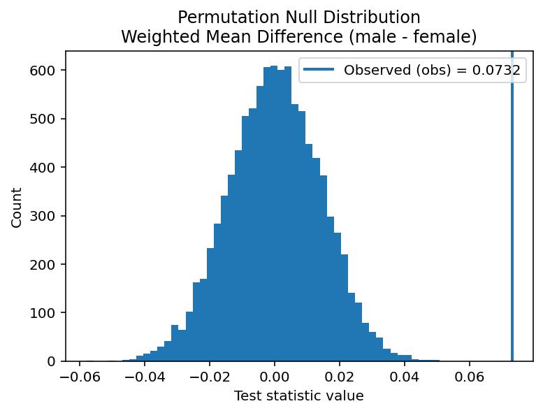
To test if there is evidence of a pro-male gender bias in this dataset, I performed a one- sided permutation test with the difference in weighted means as my test statistic. In this context, “pro-male gender bias” is defined as a higher (weighted) average rating for male professors. A permutation test was chosen to account for the fact that the ratings data is highly left-skewed, while the weighted mean difference was used as a test statistic to account for the variability in the number of ratings per professor. When considered against an observed weighted mean ratings difference (male-female) of 0.0732, this one-tailed permutation testing yielded a p value of 0.0001 for the null hypothesis that there is no pro-male gender bias in this dataset.

Given that my p value is .0001, I conclude that there is evidence of pro-male gender bias in this dataset. 

Is there a gender difference in the spread (variance/dispersion) of the ratings distribution?  

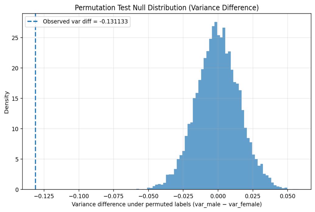
To assess if there is a gender difference in the spread of the ratings distributions, I first performed a KS test to analyze whether the male and female professors’ ratings distributions had similar shapes. Since the KS test yielded a significant result (p=0.000000), I chose to perform a permutation test to investigate whether this difference in distribution shape could be due to a difference in variance. The test statistic utilized was the difference in variance. When compared against an observed difference in variation (male-female) of -0.131, these two tailed permutation tests yielded a p value of 0.0001 for the null hypothesis that there is no gender difference in the variance of the ratings distributions.

Given that my p value is 0.0001, I conclude that there is evidence of a gender difference in variance of ratings distributions in this dataset. 

What is the likely size of both effects (gender bias in average rating, gender bias in spread of average rating), as estimated from this dataset?

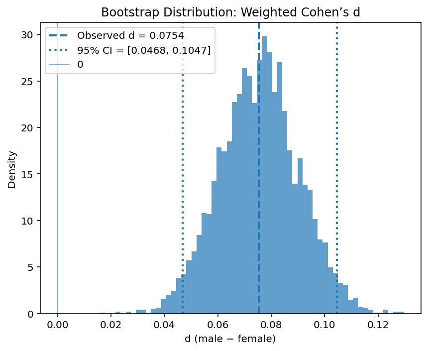
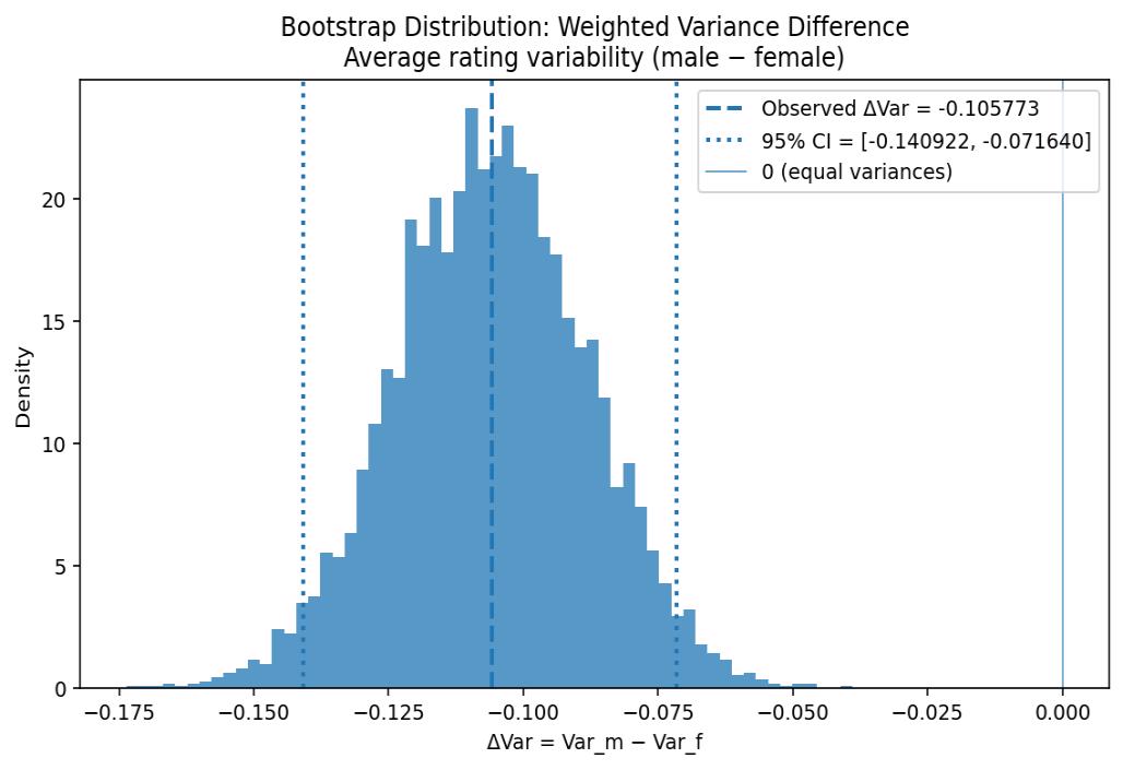
To determine the likely size of the effects of gender bias in average mean rating and gender bias in spread of average rating, I undertook a bootstrap for each while weighting the ratings based on number ratings. I did this to more heavily weight the averages which came about from a larger number of student ratings. The effect size for mean weighted rating was quantified using Cohen’s d, which was calculated to be in the range of [0.047, 0.105] with 95% confidence. The likely effect size of the variance difference was calculated to be in the range of [-0.141, -0.072] with 95% confidence.

Given that neither confidence interval for effect sizes included zero, this supports the previous testing that indicated a gender difference for both mean rating and variance of these ratings. 

Is there a gender difference in the tags awarded by students?  

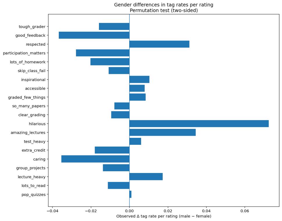
To analyze which tags exhibit a gender difference, I decided to do permutation testing on tags per rating with the test statistic of difference in tag count. I did this to determine whether the observed difference in tag counts would be likely given permutations of gender for these counts. My testing returned all tags to have a significant difference except for “pop quizzes,” which had a p value of 0.492. The top three most similar tags are “pop quizzes,” “test heavy,” and “accessible,” while the three most different tags are “hilarious,” “good feedback,” and “caring.”

Given my p-value of 0.492 for pop quizzes, I maintain that there is no gender difference for the “pop quizzes” tag and conclude that the remaining tags show evidence of gender difference. 

Is there a gender difference in terms of average difficulty? 

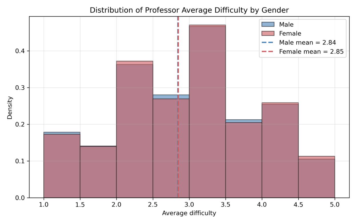
To determine if there is a gender difference in terms of average difficulty, I performed permutation tests with a test statistic of difference in (weighted) average difficulty. Although this data is much closer to a normal distribution than the ratings data, a permutation test was chosen to account for the variation in number of ratings upon which these average difficulties were based. This permutation testing yielded a p value of 0.293 as measured against an observed weighted mean difference of 0.0124.

Given that my p value is 0.293, I maintain the null hypothesis that there is no significant gender difference in terms of average difficulty in this dataset. 

Please quantify the likely size of this effect at 95% confidence.

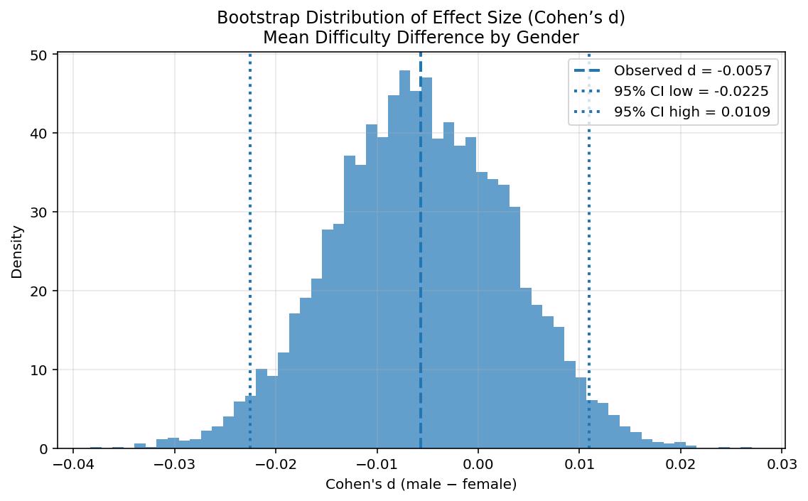
To assess the likely effect size of gender difference in course difficulty, a bootstrap was undertaken. This bootstrap calculated the likely size of Cohen’s d for difficulty rating based on gender to be within the range [-0.0225, 0.0109] at 95% confidence. The fact that the confidence interval for this effect size includes 0 is consistent with the previous testing that indicated no significant difference in course difficulty based upon the gender of the professor. 

Build a regression model predicting average rating from all numerical predictors.

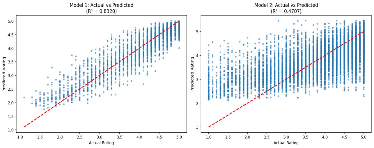
To create a regression model to predict the average rating from all numerical predictors, I devised two WLS models and employed an 80/20 test/train split. This model type was chosen because it led to higher R² and lower RMSE than Ridge and LASSO models. Regarding why I created two different models: the first one created utilized the “would take again” predictor. This yielded R²= 0.832 and RMSE = 0.348 on the test data. However, requiring datapoints to include a response in the “would take again” column reduced the sample size from over 50,000 responses to around 12,000.

For this reason, I also created a WLS model on the data without including the “would take again” column. This model was much less predictive, as it yielded R²= 0.471 and RMSE=0.689. This shows that the predictor most informative of average rating is “would take again.” However, when this was excluded, “average difficulty” is the top negative predictor and “pepper” is the top positive predictor.  

Build a regression model predicting average ratings from all tags. Which of these tags is most strongly predictive of average rating?

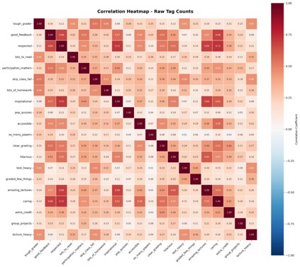
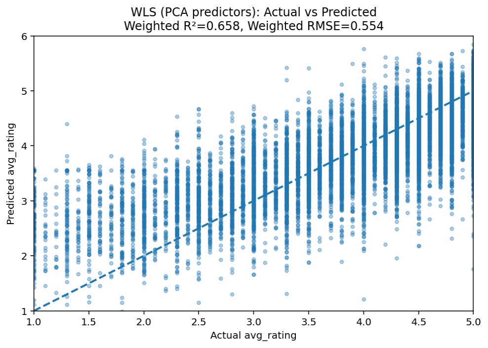
To build a regression model to predict average rating from all tags, I first did a PCA to reduce dimensionality. I did this because of collinearity between certain tags, as the model made using all predictors without PCA had a much lower R². This model achieved a test R²= 0.658 and RMSE= 0.554. The top (negative) predictor, PC1, included the tags “tough grader”, “respected”, “caring”, “inspirational”, “good feedback”, and “lecture heavy.”

Given that these tags are a part of PC1, which has the highest coefficient in this model, I conclude that variance along this tag dimension is most strongly associated with differences in average rating. Due to its higher R² and lower RMSE, this model can explain more of the variation in average ratings than the model which utilizes the numerical data.

Build a regression model predicting average difficulty from all tags. Which of these tags is most strongly predictive of average difficulty? 

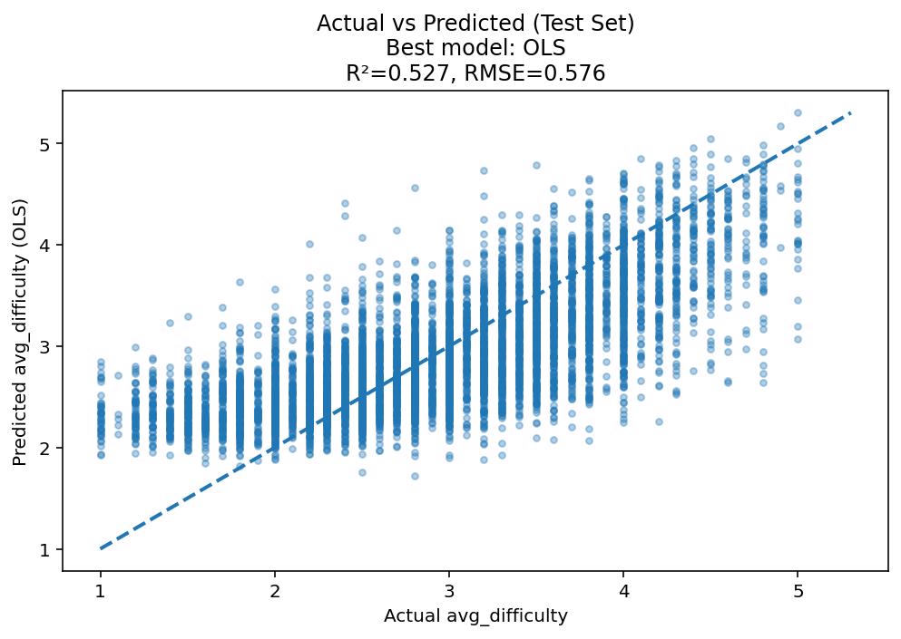
To build a regression model which predicts average difficulty, I did OLS regression. Initially I tried using PCs from my PCA that I had used previously, but this model was far less predictive, so I tested different models and ended up with OLS having the highest R² at 0.527 and lowest RMSE at 0.576. However, to achieve R² above 0.5, I had to set the minimum number of required ratings to 4. This reduced my sample size to about 32,000 but also increased the explanatory power of my model. The tag with the strongest relationship to difficulty was “tough grader.”

Given the lower R² and the need to increase the minimum ratings threshold, I conclude that the tags data hold higher explanatory power for average rating than difficulty.  

Build a classification model that predicts whether a professor receives a “pepper” from all available factors (both tags and numerical). 

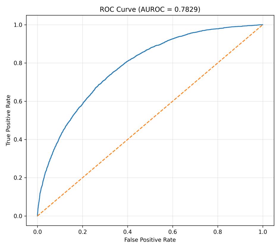
To build a classification model to predict whether a professor receives a “pepper,” I devised a logistic regression model. This was chosen because the model is classifying toward a binary outcome and will help assess the probability of each outcome. Since the proportion of ratings indicating a “pepper” is much lower than those which do not, I applied a balanced class weight to my model to address the initial class imbalance. The minimum number of ratings per input in these models was set to 1, as this is the case under which they performed best while also allowing me to utilize all valid data. My first model achieved an AUROC of 0.802 on the test data, with the strongest predictor being that of average rating. I also created a model which did not include average rating, and this model achieved an AUROC of 0.783. The top positive predictor for this model was the number of ratings, which makes sense given that the more ratings a professor has, the more likely they are to at some point receive a pepper.

These results indicate that, while average rating is highly indicative of whether a professor receives a “pepper,” one can still retain pepper prediction power without this metric.

Extra credit:

I was curious to see if there was a difference between the average professor/difficulty ratings in STEM and humanities courses, so I began by undertaking significance testing to compare these metrics between the groups. I found a very clear difference: STEM courses are rated as more difficult, while STEM professors are rated lower.

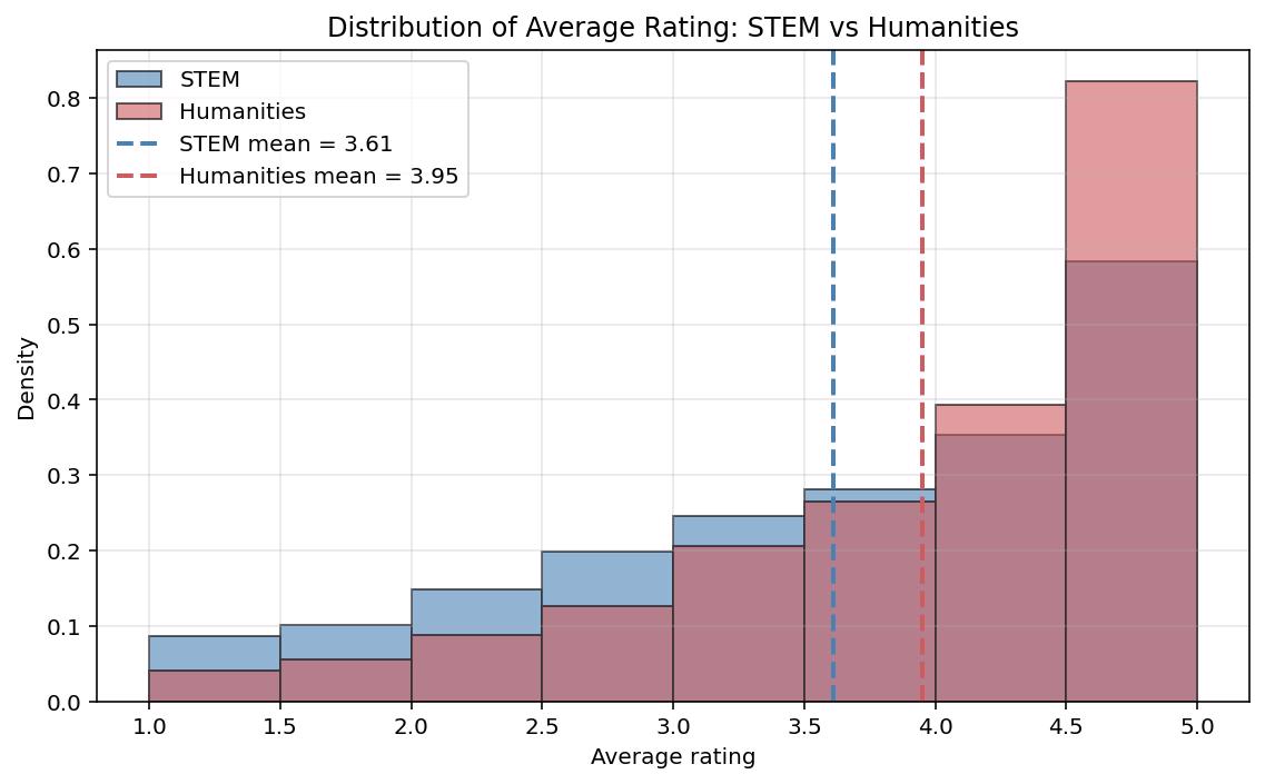
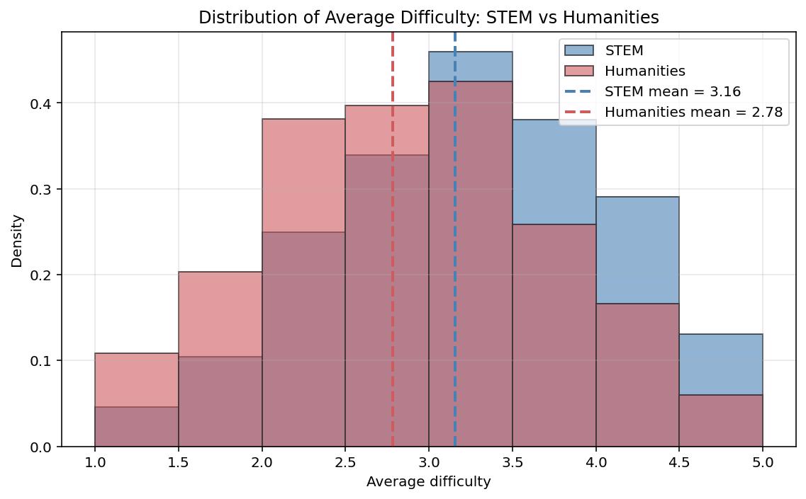
I then wanted to see if it was possible to create a model which could predict the subject-group of a course based on the metrics provided in student responses.  My results showed a relatively low AUROC based upon professor rating/ average difficulty alone, but a much higher AUROC based upon tags. When all these factors were considered, (average ratings and tags combined) the AUROC only increased by about 0.01 points from 0.829 in the tags-only model to 0.838 in the model which included all predictors. This suggests that a course’s subject is more strongly associated with the qualitative descriptors depicted via the tags, as opposed to numerical metrics such as course difficulty. 

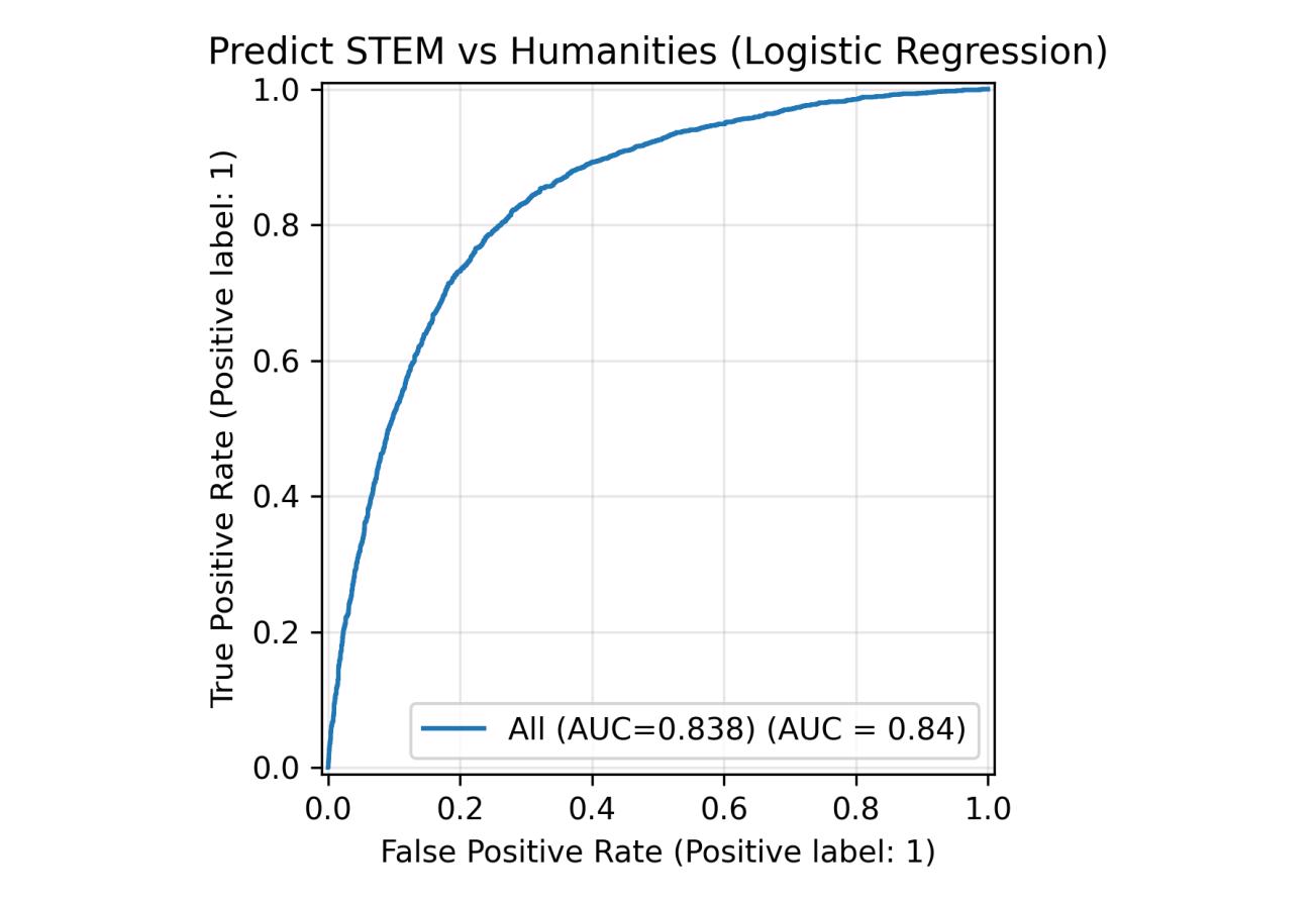
I initially found this surprising given the clear differences between professor ratings and difficulties as discovered through my initial significance testing, but it made a lot more sense when investigating the highest predictors for each type of course: “test heavy,” “lots of homework,” and “accessible” were the highest predictors for STEM courses, while “good feedback,” “lots to read,” and “so many papers”  were the highest for Humanities courses.